Distance and Parsimony methods (Part 1)

Previous class check-up

We studied the overview of phylogenetic inference and the main challenges

Learning objectives

At the end of today’s session, you will be able to

explain both algorithms to reconstruct trees: 1) based on distances and 2) based on parsimony
assess the strenghts and weaknesses of every approach
use R for tree estimation based on distances or parsinomy

Pre-class work

Optional readings: HB Ch 5-6, Baum Ch 7-8

Final project datasets: First, let’s check the different datasets that will be used in the final projects (google slides link in canvas).

Phylogenetic inference: Step 1) Choose the criterion to use: distances, parsimony, likelihood. Step 2) Search the space of trees until you find the optimum

Phylogenetic methods

	Character-based methods	Non-character-based methods
Based on an explicit model of evolution	Likelihood methods	Distance methods
Not based on an explicit model of evolution	Parsimony methods

Distance-based methods

Goal: Fit a tree to a matrix of pairwise genetic distances

Computing the distances

For every two sequences, the distance corresponds to the fraction of positions in which the two sequences differ (p-distance)
The p-distance underestimates the true genetic distance $d$
Thus, we do not use the p-distances as the pairwise distances but instead we estimate the number of substitutions that occurred by applying a specific evolutionary model

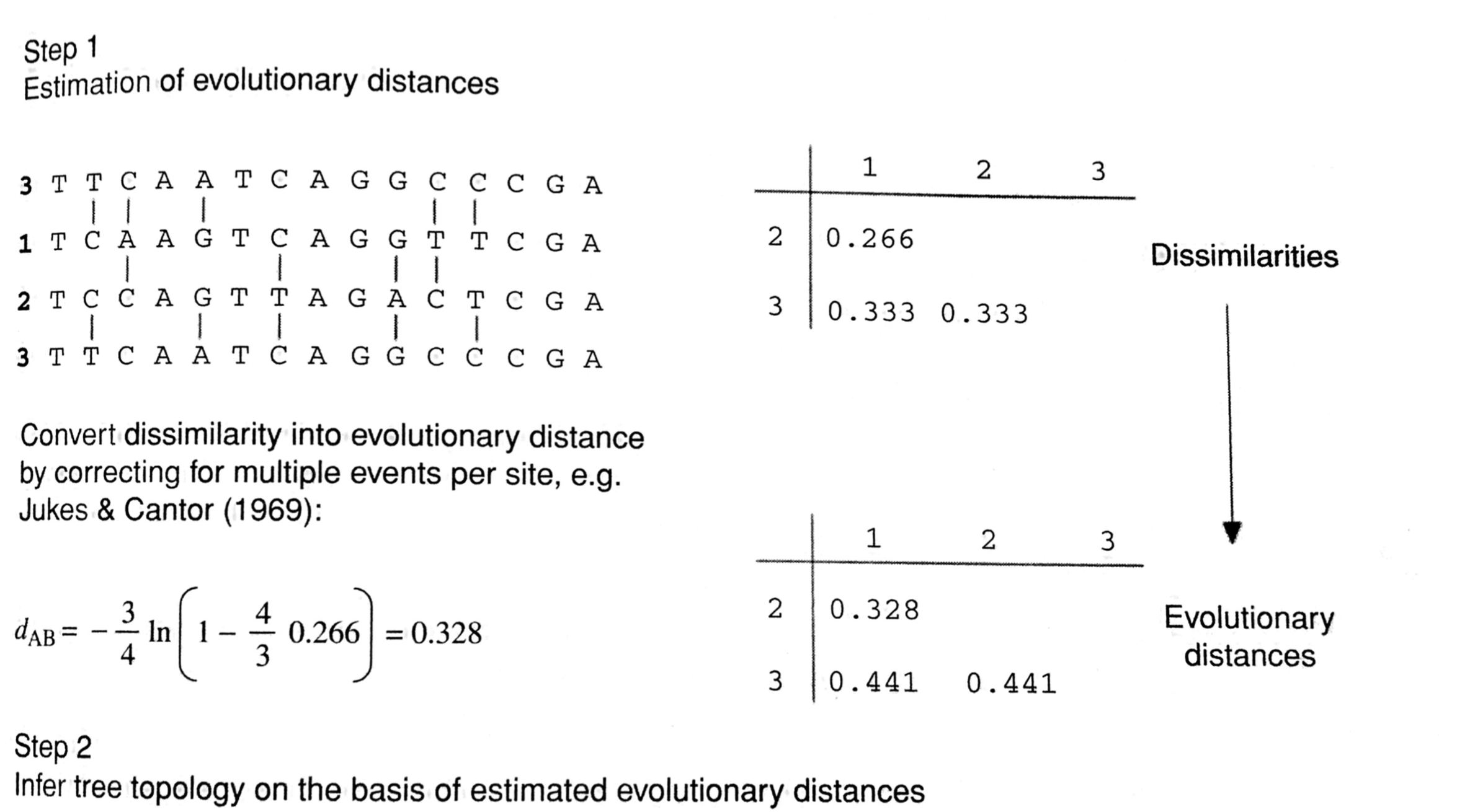
Figure 5.2 in HB 5

We will assume that the genetic distances have been estimated using an appropriate evolutionary model (more on Lectures 9 and 12)
The main distance-based tree building methods are:
- cluster analysis
- minimum evolution
Advantage of distance-based methods over parsimony or likelihood: There are algorithms that produce the optimum tree without having to search the space of trees
- Pros: You can get the tree in a scalable manner regardless of sample size
- Cons:
  - Algorithmic methods tend to be approximations, so they would approximate the optimum tree, but rarely achieve it
  - However, keep in mind that searching the space would not necessarily achieve the optimum either because many times the search is not exhaustive

Cluster analysis

Constructs ultrametric trees (rooted trees in which all the end nodes are equidistant from the root)
Only possible assuming a molecular clock:
- Zuckerland and Pauling published two fundamental papers on the evolutionary rate of proteins
- They noticed that the genetic distance of two sequences coding for the same protein on different species seems to increase linearly with divergence time
- This seems to imply that the rate of evolution for any given protein is constant: existence of a molecular clock
- This assumption is used for dating the divergences in the tree
- The molecular clock assumption aligns with the neutral theory of evolution (vs positive selection theory) and implies that deviations from clock-like behavior may reveal adaptive evolution, relaxing functional constraints or changes in effective population size
- How to test the clock hypothesis? HB 11
Constructs ultrametric trees (rooted trees in which all the end nodes are equidistant from the root)
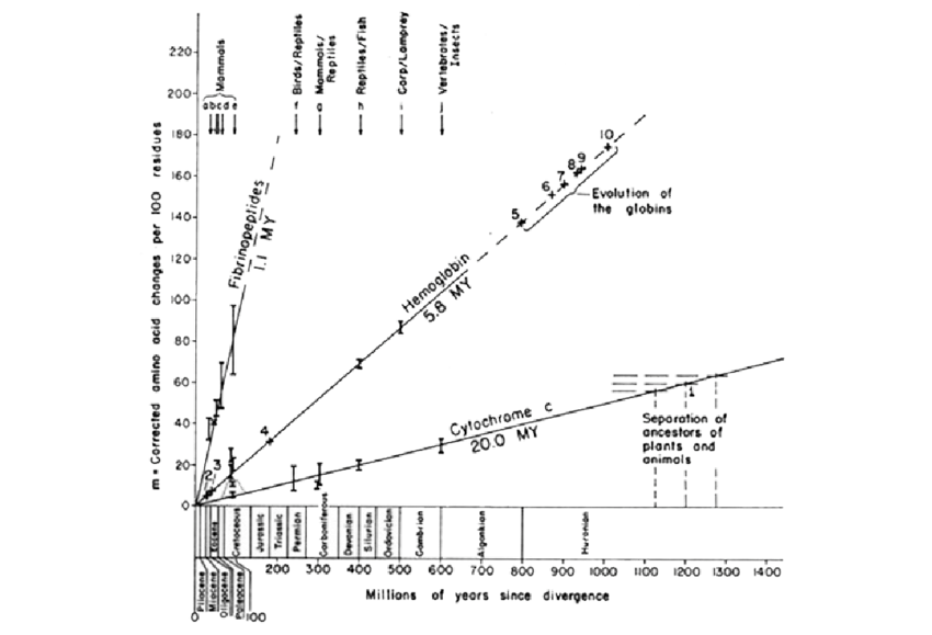
Only possible assuming a molecular clock:

Figure 11.1 in HB11

Options for Cluster Analysis:
- UPGMA: unweighted-pair group methods with arithmetic means
- WPGMA: weighted-pair group methods with arithmetic means
Cluster analysis is extremely sensitive to unequal rates in different lineages

UPGMA/WPGMA Algorithm

Input: Matrix of pairwise distances

1) Group together the two taxa with smallest distance (say A, B)

2) Compute the distance from AB to every other taxa

WPGMA: $d_{(AB)k} = \frac{d_{A,k}+d_{B,k}}{2}$ (simple average)

UPGMA: $d_{(AB)k} = \frac{N_A d_{A,k}+N_B d_{B,k}}{N_A + N_B}$ (averaged by number of taxa in the cluster)

3) Repeat until all taxa are clustered

We are not searching the space of trees here, this is an algorithm that returns a tree that agrees with the distances provided.

Cluster analysis example

In-class dynamic: (Box 5.1 in HB11) Find the WPGMA tree for the distance matrix below.

   A  B  C  D  E  F 
A
B  2  
C  4  4 
D  6  6  6
E  6  6  6  4
F  8  8  8  8  8

Watch again in YouTube video.

Minimum evolution

We want to reconstruct a tree with minimum length
The length of the tree is inferred from the genetic distances
It does not reconstruct ultrametric trees, but additive trees
An additive tree is a tree that satisfies the four-point metric condition: $d_{AB}+d_{CD} \leq max(d_{AC}+d_{BD},d_{AD}+d_{BC})$
Additive trees are always a better fit to distances under non-clock-like behavior
There is an algorithm to estimate the ME tree: neighbor-joining (NJ) (Saitou and Nei, 1987)
NJ tree is the same as the ME tree only if distances are additive to begin with, but it has been shown that the NJ tree can be very similar to the ME tree most of the times
NJ is better that UPGMA/WPGMA under unequal rates of evolution

NJ Algorithm

Input: Matrix of pairwise distances

Compute the net divergence $r$ (sum of distances) for every end node: $r_j = \sum_i d_{ij}$
Create a rate-corrected distance matrix: $M_{ij} = d_{ij} - \frac{r_i+r_j}{N-2}$
Define the new node that groups taxa $i$ and $j$ for which $M_{ij}$ is minimal (say A,B)
Compute the branch lengths from new node U to A and B: $S_{AU} = \frac{d_{AB}}{2} + \frac{r_A - r_B}{2(N-2)}$
Compute new distances from node U to every other end node: $d_{kU} = \frac{d_{Ak}+d_{Bk}-d_{AB}}{2}$
Repeat the steps

Minimum evolution example

Homework: Find the NJ tree for the distance matrix below.

   A  B   C  D  E  F 
A
B  5  
C  4  7 
D  7  10  7
E  6  9   6  5
F  8  11  8  9  8

Box 5.2 in HB11: Note that there are many errors in the book.

Solution: See this YouTube video with all the steps in the algorithm.

Distance-based methods: Main conclusions

Two steps
1. genetic distances from a p-distance and a model of evolution
2. a phylogenetic tree is constructed from the distances
Distance methods reduce the phylogenetic information to one value per pair of sequences, so many times regarded as inferior compared to character-based methods (less stat power due to the loss of info)
But unlike parsimony, they rely on an evolution model but the result will depend on which model is chosen (more on Lecture 9 and 12)
They do not have the model flexibility as likelihood-based models
Under standard conditions, NJ trees are meant to estimate accurate trees and they are very fast to be estimated
However, these methods assume the distances are accurate. Noisy distances can affect the estimated tree
Aside from the ME algorithm that aims to find the tree that minimizes the tree length, there are other ME algorithms that aim to find the tree that minimize the differences between the genetic distances and the tree distances (called OLS=ordinary least squares): $F = \sum_{i,j} (D_{ij}-d_{ij})^2$ where $D_{ij}$ are the tree distances and $d_{ij}$ are the observed genetic distances